Understanding Capital Volume II, John Fox, 1985
| "[R]eproduction on an enlarged scale . . . has nothing to do with the absolute volume of the product, . . . for a given quantity of commodities it implies merely a different arrangement or a different definition of the functions of the various elements of a given product . . " (p.510 [582]) |
At several earlier points in Capital, Marx dealt with extended reproduction -- capitalization of a portion of surplus-value -- from the perspective of an individual capital. The analysis of extended reproduction grows more complex when undertaken from the standpoint of the aggregate social capital. It becomes necessary to account not only for the individual capitalist's ability to increase the scale of production (through the accumulation of potential money capital), but as well for the ability of the economy as a whole to sustain an increase by supplying new real elements of productive capital ("virtually additional productive capital").
Marx's great achievement in the concluding chapter of Volume II is his demonstration of the possibility of extended reproduction on an economy-wide basis. Indeed, this demonstration is the primary purpose of the chapter. In the course of his investigation, Marx lays the foundation for further formal study of capitalist growth. Yet, his exposition in this chapter is difficult to follow, largely because results are expressed in the form of numerical examples, without general (i.e., algebraic) statement. To render Marx's treatment of extended reproduction more transparent, we shall formalize his presentation, at the same time adhering closely to his formulation. (A little of this sort of formalization was done in the summary of the preceding chapter.) Formalization is clearly in the spirit of Marx's Capital, for Marx was a great pioneer in the application of mathematics to the study of economy and society.
Marx develops his analysis of extended reproduction in the
context of the two department model: as before, means of production are
produced in Department I, and articles of consumption in Department II.
Because under extended reproduction the scale of production increases
from year to year, we write the basic value equations of the two
department model in the following format:
| Department I | C'1t = c1t + v1t + s1t |
| Department II | C'2t = c2t + v2t + s2t |
The symbols C', c, v, and s have their previous meanings, but each now has a double subscript: the first subscript (1 or 2) gives the department; the second subscript, t, indicates the year (and takes on the value 1 for the first year, 2 for the second, 3 for the third, etc.).
Under extended reproduction, part of the surplus-value produced in a given year is capitalized; that is, rather than being spent in its entirety as revenue for the capitalists' personal consumption, a portion of surplus-value is invested in new elements of productive capital (new means of production and labor-power). Let pl represent the rate of capitalization of surplus-value in Department I -- the proportion of surplus-value that capitalists in Department I invest in new productive capital. pl, then, must be between zero and one: if it is equal to zero, we have simple reproduction; it cannot quite reach one, for then the capitalist class would starve, that is, consume nothing. Similarly, p2 represents the rate of capitalization of surplus-value in Department II. pl and p2 are not necessarily identical; indeed, we shall see that they generally must be different, given Marx's formulation of the extended reproduction problem. (This property should be counted as a weakness of Marx's formulation.) Note, further, that we have not attached a time subscript to pl and p2. This is because, in Marx's formulation, pl and p2 stabilize; the stable values of pl and p2 for his example will be derived below.
When surplus-value is capitalized, part of it is invested as constant capital in new material means of production, and the rest as variable capital in new labor-power. How capitalized surplus-value is divided between these two components depends on the value composition of capital. Marx usually expresses the value composition of capital as a ratio, c/v. Here, we shall express the value composition :as the proportion of constant capital, k = c/(c + v), which conveys the same information, but is in a more convenient mathematical form for present purposes. In Department I, we have k1 = c1/(c1 + v1), and in Department II, k2 = c2/(c2 + v2). Note that we have omitted the time subscript here, to emphasize the point that although the amounts of constant and variable capital change over time, their proportions do not change in Marx's formal treatment of extended reproduction. It is, perhaps, unnecessary to add that the assumption of an unchanging value composition of capital, is a simplification that Marx did not regard as realistic. We should keep in mind Marx's main purpose in the present chapter: to demonstrate the logical possibility of extended reproduction, and to explore some of its properties, not to describe in detail the actual course of capital accumulation. Note, furthermore, that Marx permits a different composition of capital in the two departments; in his first illustration these quantities in fact differ, while in the second illustration they are identical.
We shall also find it convenient to have symbols for the rate of profit in each department. Marx's illustrations assume that the rate of surplus-value (s/v) is the same in the two departments. Because the compositions of capital may differ, however, the rates of profit r = s/(c + v) may differ as well. We shall let r1 represent the rate of profit in Department I, and r2 that in. Department II. The various symbols are summarized in Table 6.
Table 6. Summary of Symbols Employed
| Department I | Department II | |
| Value of Product, Year t | C'1t | C'2t |
| Constant Capital, Year t | c1t | c2t |
| Variable Capital, Year t | v1t | v2t |
| Surplus-Value, Year t | s1t | s2t |
| Capitalization Rate | p1 | p2 |
| Composition of Capital | k1 | k2 |
| Rate of Profit | r1 | r2 |
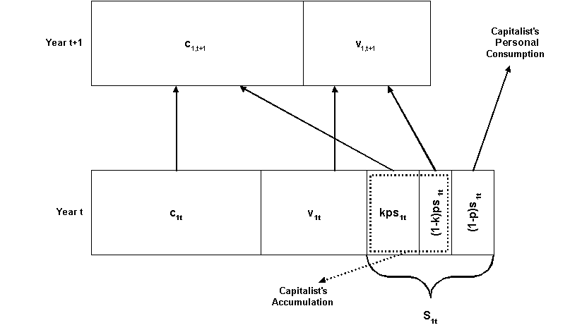
When accumulation of capital takes place, as we have mentioned, part of the surplus-value is used to purchase additional elements of constant and variable capital. In Department I, for example, in year t, p1s1t is capitalized for the next year; of this newly capitalized surplus-value, k1p1s1t goes to augment constant capital, and the remainder, (1 - k1)p1s1t , to variable capital. Similar relations hold in Department II. Thus we have the following results (where, e.g., c1,t+1 is the constant capital in Department I in year t + 1):
| Department I |
| c1,t+1 = c1t + k1p1s1t |
| v1,t+1 = v1t + (1 - k1)p1s1t |
| Department II |
| c2,t+1 = c2t + k2p2s2t |
| v2,t+1 = v2t + (1 - k2)p2s2t |
The relation of year t's product in Department I to capital advanced in this department in year t + 1 is shown schematically in Figure 9.
Figure 9. Capital Accumulation in Department I
A similar figure could be drawn for Department II.
For accumulation to be possible, next year's demand for additional constant capital must be met out of the present year's production of Department I. Of course, more labor-power is required as well, and Marx dealt at length with this topic in his discussion of the general law of capitalist accumulation in Volume I (Chapter 25); this new labor-power requires additional subsistence goods from Department II. Further, since not all surplus-value is expended as revenue for the capitalists' consumption, the demand for Department II's output is correspondingly reduced (in comparison with simple reproduction). For instance, surplus-value spent by Department I capitalists for their own consumption is (1 - p1)s1. We have, then, the supply and demand relations shown in Table 7.
Table 7. Supply and Demand in the Model for Extended Reproduction
| Department | Supply | Demand | |
| I | C'1t= c1t + v1t + s1t | c1,t+1 + c2,t+1 = c1t + k1p1s1t + c2t + k2p2s2t | |
| II | C'2t= c2t + v2t + s2t | v1,t+1
+ v2,t+1 + (1 - p1)s1t
+ (1 - p2)s2t
=
v1t
+ v2t + (1 - k1p1)s1t
+ (1 - k2p2)s2t
[after
simplification]
|
By setting supply equal to demand in either department, we obtain the fundamental equilibrium condition of Marx's extended reproduction model, namely: v1t + s1t = c2t + k1p1s1t + k2p2s2t. As Marx points out, in extended reproduction v1 + sl becomes greater than c2.
Let us turn now to Marx's first illustration, presented on pp. 514-517 [586-589]. Marx begins this example with the following first-year value relations:
| Department I: | C'11 = c11 + v11 + s11 |
| 6000 = 4000 + 1000 + 1000 | |
| Department II: | C'21 = c21 + v21 + s21 |
| 3000 = 1500 + 750 + 750 |
Note that, as before, the first subscript represents the department (1 or 2), while the second subscript denotes the year (i.e., year 1). Since c21 is less than v11 + s11 (1500 < 1000 + 1000), the possibility for extended reproduction exists. The rates of surplus-value are identical in the two departments: both are 100 per cent. The rates of profit differ, however:
r1 = 1000/(4000 + 1000) = 1/5
r2 = 750/(1500 + 750) = 1/3.
We shall return to this point below. The compositions of capital also
differ, which is necessarily the case if the rates of surplus-value are
the same but the rates of profit are different:
k1 = 4000/(4000 + 1000) = 4/5
k2 = 1500/(1500 + 750) = 2/3.
Marx further specifies that capitalists in Department I capitalize half of surplus-value, i.e., p1 = 1/2. According to the relations explained above, we may calculate the constant and variable capital employed in Department I during the second year:
c12 = c11 + k1p1s11 = 4000 + (4/5)(1/2)1000 = 4400
v12 = v11 + (1 - k1)p1s11 = 1000 + (1/5)(1/2)1000 = 1100
Marx next (implicitly) determines p2 from the equilibrium condition:
v11 + s11 = c21 + k1p1s11 + k2p2s21
1000 + 1000 = 1500 + 400 + (2/3)p2(750).
Solving, we get p2 = 1/5. Now we may calculate the constant and variable capital of Department II for the second year:
c22 = c21 + k2p2s21 = 1500 + (2/3)(1/5)750 = 1600
v22 = v21 + (1 - k2)p2s21 = 750 + (1/3)(1/5)750 = 800
The second year production value relations are, therefore:
C'12
=
c12 + v12 + s12
6600 =
4400 1100 1100
C'22 = c22
+ v22 + s22
3200 1600
800 800
Note that Department I has grown by 10 per cent [(6600 - 6000)/6000 = 0.1], while Department II has expanded by 6.7 per cent [(3200 - 3000)/3000 = 0.067]. Marx states that accumulation takes place more rapidly in Department II, but this is clearly incorrect: (1) being larger, Department I accumulates more capital; (2) the rate of accumulation is also larger in Department I, although this is an artifact of the numerical example, and, as we shall see, happens only in the first year; (3) the rate of capitalization of Department I is greater than that of Department II.
Constant and variable capital for year three in both departments may be calculated by the same method as used above. For Department I, we have:
c13 = c12
+ k1p1s12
= 4400 + (4/5)(1/2)1100 = 4840
v13 = v12
+ (1 - k1)p1s12=
1100 + (1/5)(1/2)1100 = 1210.
From the equilibrium condition:
v12 + s12
= c22
+ k1p1s12
+ k2p2s22
1100 + 1100 = 1600 + 440 + (213)p2(800)
p2 = 3/10.
And for Department II:
c23 = c22
+ k2p2s22
= 1600 + (2/3)(3/10)800 = 1760
v23 = v22
+ (1 - k2)p2s22
= 800 + (1/3)(3/10)800 = 880.
Thus, the value production relations for the third year are:
C'13 =
c13 + v13
+ s13
7260 = 4840 +
1210 + 1210
C'23 = c23
+ v23 + s23
3520 = 1760 + 880 + 880
Note that both departments have grown by 10 per cent from the second to the third year. In fact, the system has stabilized from the second year onward: each department grows annually by 10 per cent; and the value of p2 remains at 3/10. Years one through four of Marx's first illustration are summarized in Table 8.
Table 8. Marx's First Example of Extended Reproduction
| Department I | Department II | |||||||||||||||
| t | C'1t | = | c1t | + | v1t | + | s1t | C'2t | + | c2t | + | v2t | + | s2t | p2 | |
| 1 | 6000 | 4000 | 1000 | 1000 | 3000 | 1500 | 750 | 750 | 0.2 | |||||||
| 2 | 6600 | 4400 | 1100 | 1100 | 3200 | 1600 | 800 | 800 | 0.3 | |||||||
| 3 | 7260 | 4840 | 1210 | 1210 | 3520 | 1760 | 880 | 880 | 0.3 | |||||||
| 4 | 7986 | 5324 | 1331 | 1331 | 3872 | 1936 | 968 | 968 | ||||||||
The stabilized rates of growth for the two departments of Marx's model must be the same -- otherwise the relations between the departments would be disrupted. From this consideration, we may derive the relationship between the stabilized rates of capitalization of surplus-value in the two departments. Let g1 be the stabilized annual growth rate of Department I and g2 that of Department II. By definition of an annual growth rate, we have for Department I:
| g1 | = | (capital in year t+1) -
(capital in year t) capital in year |
| = | (c1,t+1
+ v1,t+1) - (c1t + v1t) c1t + v1t |
|
| = | (c1t +
v1t + p1s1t)
- (c1t
+ v1t) c1t + v1t |
|
| = | p1 s1t
= p1r1 c1t + v1t |
where, recall, r1 is the rate of profit in Department I. By similar reasoning applied to Department II: g2 = p2r2. Since g1 and g2 must be the same, we obtain p1r1 = p2r2 or p1/p2 = r2/r1. In words, the ratio of rates of capitalization is the inverse of the ratio of rates of profit. For Marx's first illustration, p1 = 1/2, r1 = 1/5, and r2 = 1/3. Thus, the stabilized rate of capitalization for Department II is p2 = 3/10, the result that we obtained previously but more tediously by examining the year to year progress of accumulation. These relations follow from Marx's model, but they are not of intrinsic interest.
Further exploration of the model would take us too far afield from Marx's exposition. Moreover, there are considerations introduced in the third volume of Capital that might be incorporated in the formal treatment of reproduction. The analysis of Marx's second illustration of extended reproduction follows the same principles as the first, and is left as an exercise for the reader.